 solee
solee
Style Transfer(1) - 'A Neural Algorithm of Artistic Style'로 Style transfer 맛보기
0. Style Transfer란?
Style Transfer란 2개의 이미지(content, style)를 새로운 하나의 이미지로 구성할 수 있는 방법입니다.
새로운 이미지의 주된 내용과 형태는 content image, 스타일과 표현 기법은 style image와 유사하도록 만드는 것이 목표입니다.
신경망을 이용해 만들어 Neural Style Transfer라고도 불리며 짧게 NST라고도 합니다.
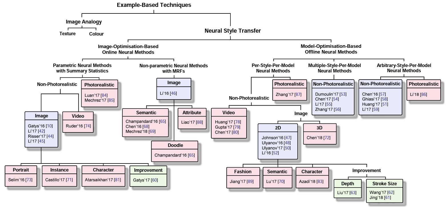 위의 그림과 같이 NST는 크게 이미지 최적화 방법과 모델 최적화 방법으로 나눌 수 있습니다.
그림은 Neural Style Transfer: A Review 에서 확인하실 수 있습니다.
이미지 최적화 방법
- ImageNet과 같은 데이터를 미리 학습된 모델을 이용해 style image와 content image의 특징을 추출한 후 새롭게 만들어지는 이미지의 특징이 추출된 두 특징과 비슷해지도록 이미지를 최적화하는 방법입니다.
- 이미지 특징을 비교하기 위해서 feature map, gram matrix 등을 사용합니다.
- 이미지 2개만으로 가능하다며 빠르다는 장점이 있지만 style image, content image를 바꾼다면 최적화 과정을 다시 진행해야 한다는 단점이 있습니다.
모델 최적화 방법
- GAN(Generative Adversarial Network)이 대표적인 모델 최적화 방법으로 입력된 두 도메인 간 변환이 가능한 모델을 학습하는 방법입니다.
- 모델을 학습한 이후에는 도메인의 새로운 input 이미지에 대해 predict만 하기에 여러 이미지를 처리하더라도 적은 시간이 소요되나 모델의 도메인 단위의 학습인만큼 많은 데이터를 필요 하다는 단점이 있습니다.
1. A Neural Algorithm of Artistic Style
A Neural Algorithm of Artistic Style은 이미지 최적화 방법을 사용한 Style transfer를 소개한 논문입니다.
Convolution Neural Network(CNN) 모델을 이용해 콘텐츠와 스타일의 표현이 분리 가능하며 두 표현을 조작하여 새로운 이미지를 만드는 것이 목표입니다.
이를 위해 style image에서는 style 특징을, content image에서는 content 특징을 분리해야 하며 분리한 특징들을 새로운 이미지를 업데이트하며 특징을 잘 표현할 수 있도록 해야 합니다.
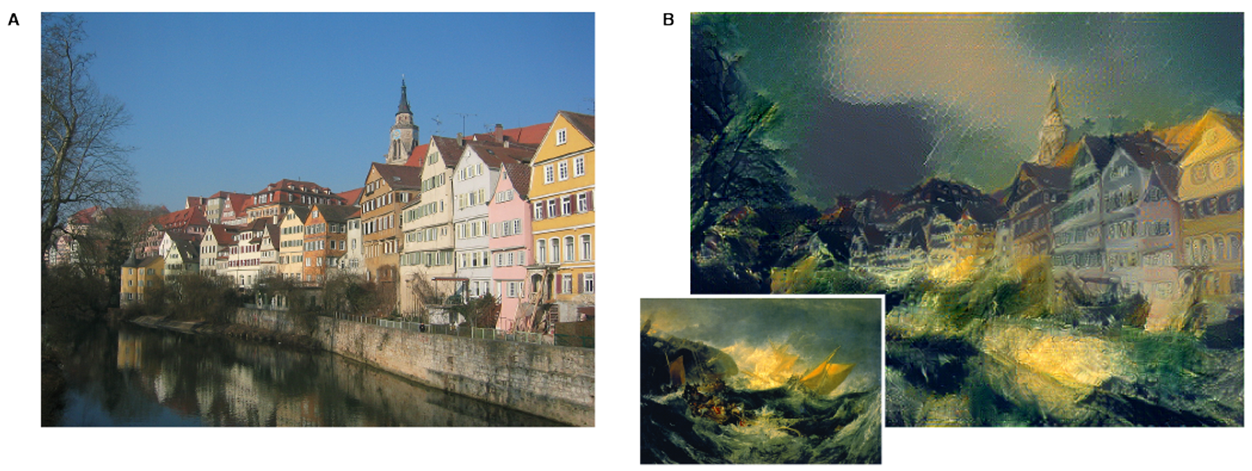
우리의 목표는 위와 같이 style과 content 특징을 하나의 이미지에 담아내는 것입니다.
어떤 방법으로 이미지가 업데이트 되는지 코드와 함께 하나하나 알아가봅시다!
2. Method
2.1. Model(VGG)
논문에서 언급된 VGG19를 사용했습니다. 논문에서 사용한 모델은 VGG 모델을 변형한 것으로 FC layer를 없애고 max pooling 대신 average pooling을 사용했다 합니다.
class VGG(nn.Module):
    def __init__(self, required_grad=False):
        super(VGG, self).__init__()
        vgg_pretrained = models.vgg19(pretrained=True).features

        # MaxPooling -> AvgPooling
        idx_pooling = [4, 9, 18, 27, 36]
        for idx in idx_pooling:
            vgg_pretrained[idx] = nn.AvgPool2d(kernel_size=2, stride=2, padding=0, ceil_mode=False)

        # output
        self.conv1_1 = nn.Sequential()
        self.conv2_1 = nn.Sequential()
        self.conv3_1 = nn.Sequential()
        self.conv4_1 = nn.Sequential()
        self.conv5_1 = nn.Sequential()

        for x in range(2):
            self.conv1_1.add_module(str(x), vgg_pretrained[x])
        for x in range(2, 7):
            self.conv2_1.add_module(str(x), vgg_pretrained[x])
        for x in range(7, 12):
            self.conv3_1.add_module(str(x), vgg_pretrained[x])
        for x in range(12, 21):
            self.conv4_1.add_module(str(x), vgg_pretrained[x])
        for x in range(21, 30):
            self.conv5_1.add_module(str(x), vgg_pretrained[x])

        if not required_grad:
            for param in self.parameters():
                param.required_grad = False

    def forward(self, x):
        conv1_1 = self.conv1_1(x)
        conv2_1 = self.conv2_1(conv1_1)
        conv3_1 = self.conv3_1(conv2_1)
        conv4_1 = self.conv4_1(conv3_1)
        conv5_1 = self.conv5_1(conv4_1)
        vgg_output = namedtuple("vgg_output", ['conv1_1', 'conv2_1', 'conv3_1',
                                               'conv4_1', 'conv5_1'])
        output = vgg_output(conv1_1, conv2_1, conv3_1, conv4_1, conv5_1)
        return output
parameter의 required_grad 값을 False로 설정해 모델의 학습을 막아야 합니다. 이미지 최적화인 방법임을 확인할 수 있습니다![]()
위에서 설명한 것처럼 FC Layer는 사용하지 않으며 max pooling을 average pooling으로 바꾸었습니다.
conv1_1, conv2_1, conv3_1, conv4_1, conv5_1로 나누어 결과로 보내는 것은 아래에서 설명될 Loss를 계산할 시 layer 별 Loss 값을 계산하기 때문입니다.
2.2. Content Loss
\(\mathcal{L}_{content}(\vec p, \vec x, l) = \frac{1}{2} \sum _{ij}(F^l _{ij} - P^l _{ij})^2\)
p = 입력한 content image
x = 만들고자 하는 결과 이미지
P = p의 feature map
F = x의 feature map
Content Loss는 feature map 간의 차를 loss로 계산합니다.
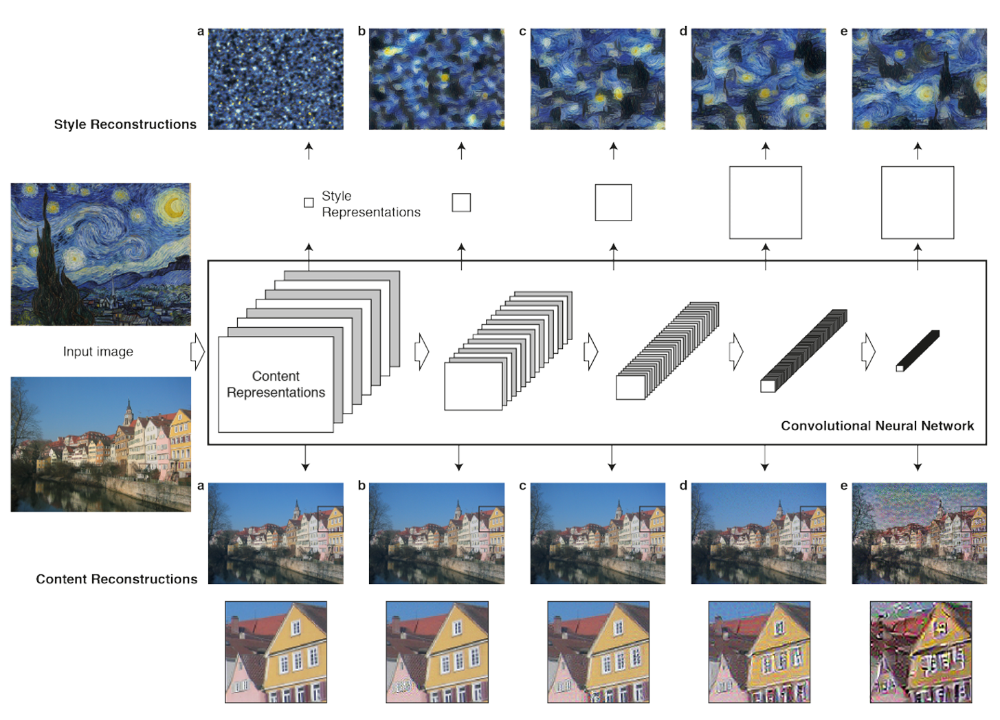
feature map은 activation map이라고도 불리며 filter의 계산 값입니다. 위의 그림에서 왼쪽의 빨간 사각형이 filter를 의미합니다.
filter가 입력 이미지 또는 이전 filter의 결과 값을 입력받아 stride 값만큼 이동하며 결과 feature map 값을 계산합니다.
수식의 $P^l_{ij}$는 l번째 레이어에서 i번째 필터의 j번째 output를 의미합니다.
class ContentLoss(nn.Module):
    def __init__(self, content_feature):
        super(ContentLoss, self).__init__()
        self.content = content_feature

    def forward(self, x):
        loss_method = nn.MSELoss()
        x_len = len(x)
        loss_total = torch.tensor(0.0, requires_grad=True)

        for layer_idx in range(x_len):
            loss_total = loss_total + loss_method(x[layer_idx], self.content[layer_idx])
        loss_total = loss_total / 2
        return loss_total
content 이미지의 feature map은 학습하는 동안 변하지 않으므로 미리 계산된 content 이미지의 feature map을 입력으로 받아 계산에 소요되는 시간을 줄였습니다.
Content Loss는 feature map 간의 평균제곱오차값이므로 MSELoss를 사용해 쉽게 구할 수 있으며 layer 별 MSELoss 값을 구한 뒤 더함으로써 ContentLoss를 계산할 수 있습니다.
2.3. Style Loss
\(\mathcal L_{style}(\vec a, \vec x) = \sum^L_{l=0}w_lE_l = \sum^L_{l=0}w_l \frac{1}{4N^2_lM^2_l} \sum _{ij}(G^l _{ij} - A^l _{ij})^2\)
$w_l$ = 레이어 별 가중치
$G^l_{ij}$ = 만들고자 하는 이미지 x의 레이어 l에서의 gram matrix
$A^l_{ij}$ = 스타일 이미지의 레이어 l에서의 gram matrix
$N_l$ = 레이어 l에서의 필터의 개수
$M_l$ = 레이어 l에서의 feature map의 크기(height * width)
Style Loss를 이해하기 위해서는 gram matrix를 알아야 합니다.
gram matrix는 feature map 별 분산이 비교가능한 Covariance Matrix의 형태를 띄우고 있는 것이 특징으로 수식은 아래와 같습니다.
\(G^l_{ij} = \sum_k F^l _{ik}F^l _{jk}\)
$F^l _{ik}$ = l번째 layer에서의 flatten된 이미지의 k번째 픽셀의 i번째 필터의 결과 값
아이공님의 Gram matrix 정리, 홍정모님의 Gram matrix 설명로 이해에 도움을 받을 수 있습니다![]()
class StyleLoss(nn.Module):
    def __init__(self, style_feature):
        super(StyleLoss, self).__init__()
        self.style = style_feature

    def gram_matrix(self, x):
        b, ch, h, w = x.shape
        x = x.view(b, ch, h*w)
        x_t = x.transpose(1, 2)
        gram = x.bmm(x_t)
        return gram

    def forward(self, x):
        x_len = len(x)
        loss_total = torch.tensor(0.0, requires_grad=True)
        loss_method = nn.MSELoss()

        for layer_idx in range(x_len):
            style_gram = self.gram_matrix(self.style[layer_idx])
            x_gram = self.gram_matrix(x[layer_idx])

            b, ch, h, w = x[layer_idx].shape
            loss_layer = loss_method(x_gram, style_gram) / (4 * ch**2 * (h*w)**2)
            loss_total = loss_total + loss_layer/x_len

        return loss_total
style 이미지의 feature map 또한 content 이미지의 feature map과 마찬가지로 학습하는 동안 변하지 않으므로 미리 계산된 style 이미지의 feature map을 입력으로 받습니다.
style loss은 gram matrix 간의 평균제곱오차값이므로 content loss와 마찬가지로 MSELoss를 사용했습니다.
layer 별 loss 값을 구한 뒤 $N_l^2$, $M_l^2$ 값으로 나누어 더해줌으로써 style loss 값을 구할 수 있습니다.
2.4. Total Loss
\(\mathcal L_{total}(\vec p, \vec a, \vec x) = \alpha \mathcal L_{content}(\vec p, \vec x) + \beta \mathcal L_{style} (\vec a, \vec x)\)
최종 Loss 값은 앞에서 구한 style loss와 content loss를 더해주어야 합니다!
이때 $\alpha$와 $\beta$ 값 조절로 style 이미지와 content 이미지 중 어느 것에 중점을 둘지 조절할 수 있습니다.
논문에서는 $ \alpha / \beta$ 의 비율은 $ 1 \times 10^{-3} $ 이나 $1 \times 10^{-4}$ 로 설정했다고 합니다.
style_loss = style(result) * style_weight
content_loss = content(result) * content_weight

loss = style_loss + content_loss
3. Result
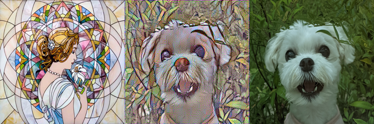
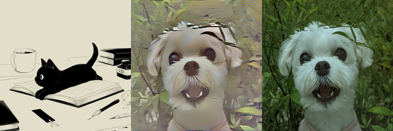
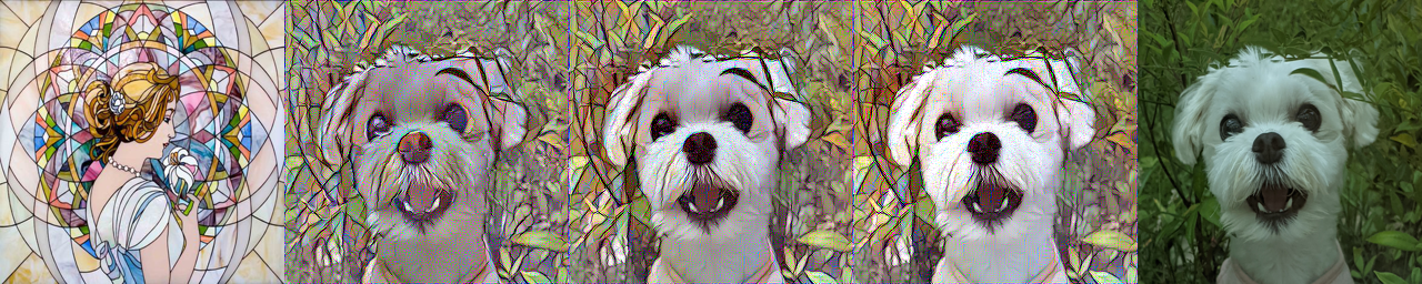
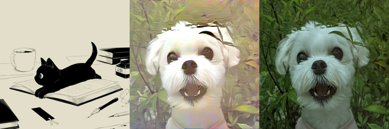
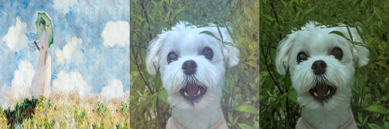
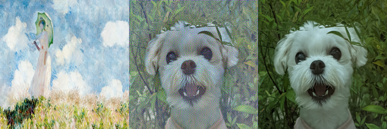 3가지 스타일 이미지를 사용해 코드를 실행한 결과 위와 같은 결과를 얻을 수 있었고 왼쪽부터 순서대로 style 이미지, 결과 이미지, content 이미지입니다.
결과 이미지가 content 이미지의 내용도 담고 있는 것을 확인할 수 있지만 스타일의 경우 style 이미지의 컬러 톤을 가져온다는 느낌은 있지만 스타일 자체를 따라한다는 느낌은 받기 어려웠습니다![]()
이미지 별 $ \alpha / \beta$ 비율을 조절해 조금씩은 더 나아보이는 결과를 얻을 수 있었지만 이미지마다 비율 값을 조금씩 조절하기에는 시간이 너무 오래 소요되는 느낌을 받았습니다.
따라서 단순한 비율 조절 외에 결과를 더 좋게 하기 위한 최적화 과정을 진행했습니다.
4. 최적화
4.1. layer weight
layer_weight = [0.5, 1.0, 1.5, 3.0, 4.0]

# content loss의 forward 부분입니다
for layer_idx in range(x_len):
    loss_total = loss_total + loss_method(x[layer_idx], self.content[layer_idx]) * self.weight[layer_idx]
loss_total = loss_total / 2
사용된 VGG19에는 총 5 layer가 있어 기존에는 loss를 계산 시 layer loss 값을 모두 더해 계산합니다. 여기에 layer 별 weight 값을 추가해 깊은 layer 일수록 weight 값이 높아 loss 계산에 더 큰 영향을 미칠 수 있도록 했습니다.
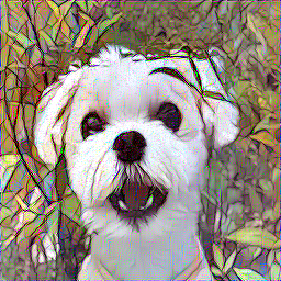
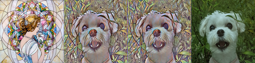 위 사진의 왼쪽에서 2번째 사진이 기존 결과, 왼쪽에서 3번째 사진이 layer weight를 추가한 결과입니다.
두 사진의 비교했을 때 layer weight를 추가한 쪽이 좌측 풀잎들이 더 잘게 나누어져 스테인드 글라스의 느낌을 잘 내고 있다고 판단해 epoch 값을 300, 1000, 2500까지 늘려가며 결과를 확인해보았습니다.
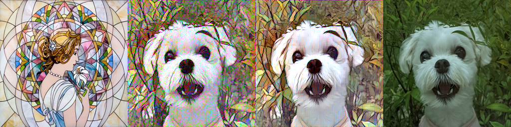
 왼쪽부터 순서대로 epoch 300, 1000, 2500이며 epoch이 늘어날 수록 style 이미지의 밝기가 반영되어 더 밝아지는 걸 확인할 수 있었습니다.
4.2. regularization
layer weight를 추가하고 epoch을 늘려 style 이미지가 더 반영된다고 느껴졌으나 결과 이미지에 전반적으로 밝게 튀는 노이즈들이 확인되었습니다.
Tensorflow core에서 관련된 문제를 해결하는 것을 확인해 total variance loss(tv loss)를 사용해 이미지의 고주파 구성요소에 대한 regularization 과정을 추가했습니다. \(\mathcal L_{tv} = w_t \times (\sum^3 _{c=1}\sum^{H-1} _{i=1}\sum^W _{j=1}(x _{i+1, j, c} - x _{i, j, c})^2 + \sum^3 _{c=1}\sum^H _{i=1}\sum^{W-1} _{j=1}(x _{i, j+1, c} - x _{i, j, c})^2)\)
def total_variation_loss(img):
     bs_img, c_img, h_img, w_img = img.size()
     tv_h = torch.pow(img[:,:,1:,:]-img[:,:,:-1,:], 2).sum()
     tv_w = torch.pow(img[:,:,:,1:]-img[:,:,:,:-1], 2).sum()
     return (tv_h+tv_w)/(bs_img*c_img*h_img*w_img)
tv loss는 이미지를 입력받아 수직/수평으로 인접한 픽셀에 대한 픽셀 값 차이의 제곱 합으로 계산할 수 있습니다.
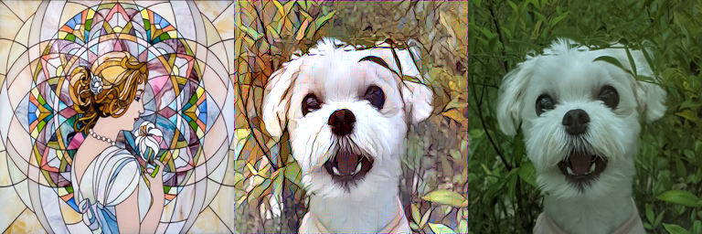
tv loss 적용 후 튀어 보이는 artifact가 줄어들여 결과 이미지가 부드러워져 선명도가 높아진 것을 확인할 수 있습니다 ![]()
5. 최종 결과
최적화 과정까지 진행 후 여러 style과 content 이미지를 넣어 확인한 결과들입니다 ![]()
최종 코드는 github에서 확인하실 수 있습니다 ![]()