 solee
solee
MUNIT(2) - 논문 구현
이전 글인 MUNIT(1) - 논문 리뷰에 이은 MUNIT 코드 구현입니다! 얼레벌레 우당탕탕 구현기임을 감안해주세요 ㅎㅅㅎ…
논문의 공식 코드는 github에서 제공되고 있습니다.
1. 데이터셋
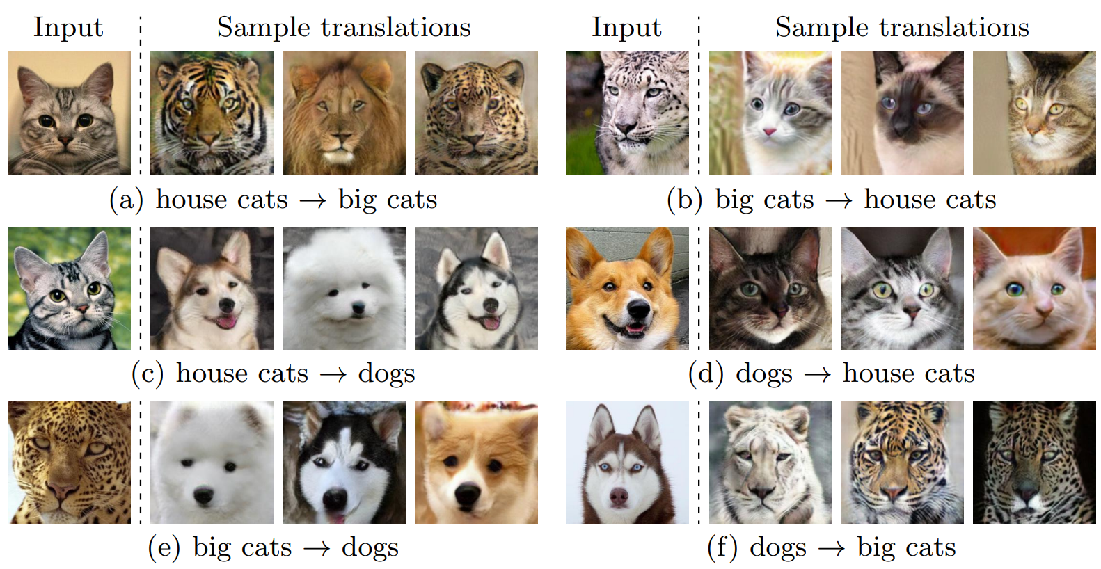
Fig.6. Animal image 변환의 결과 (MUNIT 논문)
논문에서 사용된 데이터 셋은 Edges $\leftrightarrow$ shoes/handbas, Animal image translation, Street scene images, Yosemete summer $\leftrightarrow$ winter가 있는데, 저는 그 중에서 Animal Translation dataset을 사용해 동물 간의 변환을 구현하는 것으로 목표를 잡았습니다. 이유는 하나입니다. 귀여우니까요 ![]()
![]()
![]()
![]()
MUNIT에서 Animal Translation을 수행할 때는 ImageNET의 데이터를 사용했습니다. 하지만 MUNIT의 issue에서 ImageNet 데이터셋의 저작권 때문에 사용한 데이터를 공개할 수는 없다는 것을 보게 되었습니다. 사용할 수 있는 다른 유사한 데이터셋을 찾아보다 Animal-Faces-HQ(AFHQ)를 찾게 되어 AFHQ 데이터셋을 사용했습니다. AFHQ 데이터셋을 사용해 개와 고양이 두 도메인 간 변환을 시도해보겠습니다!
AFHQ 소개
Animal-Faces-HQ(AFHQ)는 StarGAN-v2에서 공개한 데이터로 ‘dog’, ‘cat’, ‘wild’로 3개의 도메인이 있으며 3개의 도메인에 각각 약 5000장의 이미지가 포함되어 있는 데이터셋입니다. ‘dog’에는 다양한 종의 개, ‘cat’에는 다양한 종의 고양이, ‘wild’에는 여우, 치타, 호랑이, 사자 등의 육식 동물이 포함되어 있습니다.
AFHQ-v2도 공개되어 있는데 기존의 nearest neighbor downsampling이 아닌 Lanczos resampling을 이용해 더 좋은 퀄리티의 AFHQ 데이터셋이라 합니다. 두 데이터셋 모두 bash로 쉽게 다운 받을 수 있어 이용하기 용이했습니다.
# afhq
bash download.sh afhq-dataset

# afhq-v2
bash download.sh afhq-v2-dataset
AFHQ 처리
AFHQ는 ‘train’, ‘val’로 폴더가 나뉘어져 있으며 각각의 폴더 내부에 ‘dog’, ‘cat’, ‘wild’ 폴더가 존재합니다. target 인자로 어떤 폴더를 읽어올지 선택한 후 해당 폴더의 jpg 이미지 경로를 glob으로 모두 읽어오도록 구현했습니다.
데이터를 호출할 때는 idx에 맞는 self.images의 경로를 읽고 pillow로 이미지를 열어 transform을 적용한 후 이미지를 return했습니다.
class AFHQ(Dataset):
    def __init__(self, path, target, transforms=None):
        self.path_dataset = path + '\\' + target
        self.transforms = transforms
        self.images = glob(self.path_dataset + '\\*.jpg')

    def __getitem__(self, idx):
        image = Image.open(self.images[idx]).convert('RGB')

        if self.transforms:
            image = self.transforms(image)

        return image

    def __len__(self):
        return len(self.images)


transform = transforms.Compose([
  transforms.Resize((256, 256)),
  transforms.RandomHorizontalFlip(0.5),
  transforms.ToTensor(),
  transforms.Normalize((0.5, 0.5, 0.5), (0.5, 0.5, 0.5))
])

DATA_PATH = 'E:\\DATASET\\afhq\\train'

dataset_dog = AFHQ(path=DATA_PATH, target='dog', transforms=transform)
dataset_cat = AFHQ(path=DATA_PATH, target='cat', transforms=transform)

dataloader_dog = DataLoader(dataset=dataset_dog, batch_size=batch_size, shuffle=True)
dataloader_cat = DataLoader(dataset=dataset_cat, batch_size=batch_size, shuffle=True)
이미지가 제대로 들어오는 지 dataloader_dog와 dataloader_cat에서 한 장씩을 확인해보았습니다. 논문에서 batch_size=1로 저 또한 batch_size=1로 설정했기 때문에 이미지는 한 장씩 들어옵니다.
def get_plt_image(img):
    return transforms.functional.to_pil_image(0.5 * img + 0.5)

data_dog = next(iter(dataloader_dog))
data_cat = next(iter(dataloader_cat))

plt.figure(figsize=(8, 4))
plt.suptitle('Data of dog & cat')

plt.subplot(1, 2, 1)
plt.imshow(get_plt_image(data_dog[0]))
plt.axis('off')

plt.subplot(1, 2, 2)
plt.imshow(get_plt_image(data_cat[0]))
plt.axis('off')

plt.tight_layout()
plt.savefig('./history/data.png', dpi=300)
plt.show()
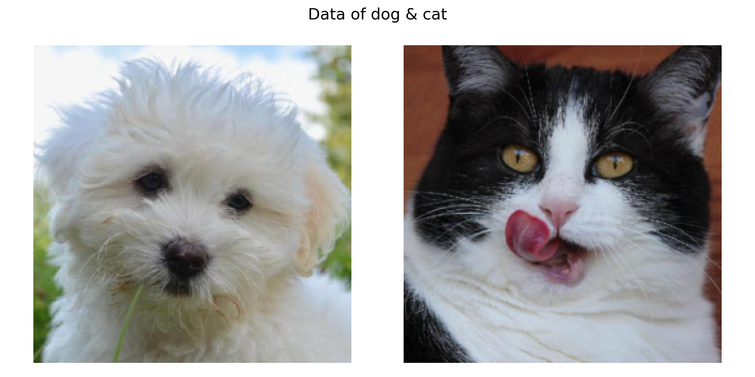
귀엽다!
2. 모델
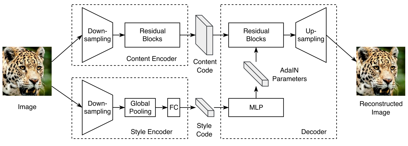
Fig.3 auto-encoder 구조
MUNIT 논문의 Fig.3과 B. Training Details에서 간략한 모델 구조를 확인할 수 있습니다. 위의 구조는 Generator에 해당하는 부분으로 이미지 생성에 대한 구조를 볼 수 있으며 여기에서 adversarial한 Discriminator가 추가되면 MUNIT의 전체 구조가 됩니다. 아래는 MUNIT 논문에서 표시된 각 모델의 구조입니다.
- Generator architecture
- Content encoder: $\mathsf{c7s1-64, d128, d256, R256, R256, R256, R256}$
- Style encoder: $\mathsf{c7s1-64, d128, d256, d256, d256, GAP, fc8}$
- Decoder: $\mathsf{R256, R256, R256, R256, u128, u64, c7s1-3}$
- Discriminator architecture : $\mathsf{d64, d128, d256, d512}$
표기법이 어디선가 봤다 했더니 CycleGAN 코드 구현 글이네요. CycleGAN과 유사한 표기와 convolution 구조를 사용합니다. 추가된 것으로는 Global average pooling을 의미하는 $\mathsf{GAP}$과 fully connected layer를 의미하는 $\mathsf{fck}$가 있으며 Decoder에 사용되는 $\mathsf{uk}$의 경우 CycleGAN과 표기는 같으나 사용하는 convolution, normalization이 달라 CycleGAN의 uk와는 모듈 간 차이가 존재합니다.
MUNIT에서 정의한 모듈 내용은 다음과 같습니다.
- $\mathsf{c7s1-k}$ : k filter와 1 stride를 가진 7x7 Convolution - InstanceNorm - ReLU
- $\mathsf{dk}$ : k filter와 2 stride를 가진 4x4 Convolution - InstanceNorm - ReLU
- $\mathsf{Rk}$ : [k filter를 가진 3x3 Convolution - InstanceNorm - ReLU] x 2 (Residual block)
- $\mathsf{uk}$ : nearest-neighbor upsampling - k filter와 1 stride를 가진 5x5 convolution - LayerNorm - ReLU
- $\mathsf{GAP}$ : Global Average Pooling
- $\mathsf{fck}$ : k filter를 가진 fully connected layer
Generator와 Discriminator에서 사용하는 $\mathsf{c7s1-k}$, $\mathsf{dk}$, $\mathsf{uk}$는 convolution-normalization-activation이라는 공통 구조를 가지고 있기 때문에 class xk를 만들어 쉽게 호출할 수 있도록 구현했습니다.
class xk(nn.Module):
    def __init__(self, name, in_feature, out_feature, norm_mode='in'):
        super(xk, self).__init__()

        model = []
        norm = [nn.InstanceNorm2d(out_feature)]
        relu = [nn.ReLU()]

        if name == 'c7s1':
            conv = [nn.Conv2d(in_feature, out_feature, kernel_size=7, stride=1, padding=3, padding_mode='reflect')]

        elif name == 'dk':
            conv = [nn.Conv2d(in_feature, out_feature, kernel_size=4, stride=2, padding=1, padding_mode='reflect')]

        elif name == 'uk':
            conv = []
            conv += [nn.Upsample(scale_factor=2, mode='nearest')]
            conv += [nn.Conv2d(in_feature, out_feature, kernel_size=5, stride=1, padding=2)]

            norm = [LayerNorm(out_feature)]

        model += conv
        model += norm
        model += relu

        self.model = nn.Sequential(*model)

    def forward(self, x):
        return self.model(x)
$\mathsf{Rk}$는 Content encoder와 Decoder에서 사용되며 이전 논문 구현글에서 사용했던 Residual block과 유사합니다. 이전 코드에서 Residual block은 instance normalization만 사용했었지만 이번 코드의 Residual block에서는 normalization 종류가 늘어 Adaptive Instance normalization이 추가되어 norm_mode 인자 값을 통해 선택할 수 있도록 구현했습니다.
Adain이라 불리는 Adaptive instance normalization은 Decoder에서만 사용되는 normalization으로 Adain에 대해서는 Decoder 부분에서 더 자세하게 설명하겠습니다. normalization을 제외하면 Residual block은 이전에 코드 구현에서 사용하던 것과 동일합니다.
class Residual(nn.Module):
    def __init__(self, in_feature, out_feature, norm_mode='in'):
        super(Residual, self).__init__()

        if norm_mode == 'in':
            norm = nn.InstanceNorm2d(out_feature)
        elif norm_mode == 'adain':
            norm = AdaptiveInstanceNorm2d()

        conv = nn.Conv2d(in_feature, out_feature, kernel_size=3, padding=1, padding_mode='reflect')
        relu = nn.ReLU()

        model = []
        for _ in range(2):
            model += [conv, norm, relu]

        self.model = nn.Sequential(*model)

    def forward(self, x):
        return x + self.model(x)
모델에서 여러 곳에 사용되는 class xk와 class Residual 먼저 코드를 살펴봤으니 다음으로는 생성 모델에 해당하는 Content Encoder, Style Encoder, Decoder와 판별 모델인 Discriminator까지 구조를 하나하나 살펴보겠습니다!
Content Encoder
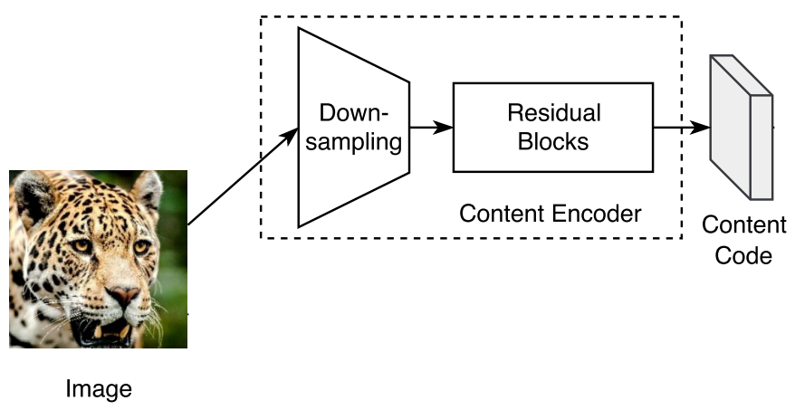
Fig.3에서 표현된 Content Encoder 부분
Content Encoder는 이미지를 입력받아 이미지의 내용을 담고 있는 Content code를 만드는 것이 목적입니다. Content Encoder의 구조는 $\mathsf{c7s1-64}$, $\mathsf{d128}$, $\mathsf{d256}$, $\mathsf{R256}$, $\mathsf{R256}$, $\mathsf{R256}$, $\mathsf{R256}$으로 Down-sampling, Residual Blocks 2단계로 이루어져 있습니다.
Down-sampling 부분은 $\mathsf{c7s1-64}$, $\mathsf{d128}$, $\mathsf{d256}$으로 위의 class xk로 객체를 만들었습니다.
Residual Blocks는 $\mathsf{R256}$, $\mathsf{R256}$, $\mathsf{R256}$, $\mathsf{R256}$으로 class Residual로 객체를 만들었습니다. Content Encoder에서는 normalization으로 Instance Normalization을 사용하므로 norm_mode 인자 값으로 ‘in’을 넣어주었습니다.
Down-sampling, Residual 과정 이후 추출된 Content Code는 batch_size=1 일 경우 [1, 256, 64, 64]의 크기를 갖습니다.
class ContentEncoder(nn.Module):
    def __init__(self):
        super(ContentEncoder, self).__init__()

        self.model = nn.Sequential(
            # Down-sampling
            xk('c7s1', 3, 64),
            xk('dk', 64, 128),
            xk('dk', 128, 256),

            # Residual Blocks
            Residual(256, 256, norm_mode='in'),
            Residual(256, 256, norm_mode='in'),
            Residual(256, 256, norm_mode='in'),
            Residual(256, 256, norm_mode='in')
        )

    def forward(self, x):
        return self.model(x)
Style Encoder
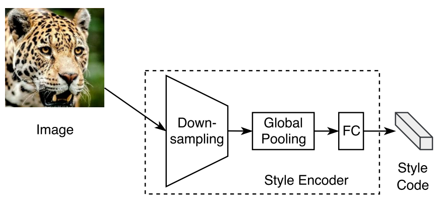
Fig.3에서 표현된 Style Encoder 부분
Style Encoder는 이미지를 입력으로 받아 이미지의 스타일을 나타내는 Style code를 출력하는 것이 목표입니다. Style Encoder의 구조는 $\mathsf{c7s1-64, d128, d256, d256, d256, GAP, fc8}$으로 Down-sampling, Global pooling, Fully connected layer 단계로 이루어져 있습니다.
Down-sampling 부분은 $\mathsf{c7s1-64, d128, d256, d256, d256}$으로 Content Encoder와 마찬가지로 class xk를 사용해 만들었습니다.
Global Average Pooling은 FC 과정 전 feature map의 모양을 [batch_size, 256, width, height]에서 [batch_size, 256, 1, 1]로 만들어 차원 수를 줄이기 위함입니다. GAP의 경우 pytorch에서 따로 함수를 주지는 않지만 3가지 구현방법이 있으며 저는 그 중 AdaptiveAvgPool2d를 사용했습니다. 구현방법은 JINSOL KIM님의 Global Average Pooling을 참고했습니다.
Fully Connected layer는 [batch_size, 256, 1, 1]인 feature map의 모양을 스타일 코드 차원 수에 맞게 [batch_size, dim_style]로 변형합니다. 논문에서 스타일 코드의 차원 수는 8로 정했으므로 nn.Linear를 사용해 스타일 코드를 [1, 8] 크기로 조정했습니다.
class StyleEncoder(nn.Module):
    def __init__(self):
        super(StyleEncoder, self).__init__()

        self.model = nn.Sequential(
            # Down-sampling
            xk('c7s1', 3, 64),
            xk('dk', 64, 128),
            xk('dk', 128, 256),
            xk('dk', 256, 256),
            xk('dk', 256, 256)
        )

        # Global average pooling
        self.gap = nn.AdaptiveAvgPool2d((1, 1))

        # FC
        self.fc = nn.Linear(256, 8)

    def forward(self, x):
        x = self.model(x)
        x = self.gap(x)
        x = self.fc(x.flatten(start_dim=1))

        return x
Decoder
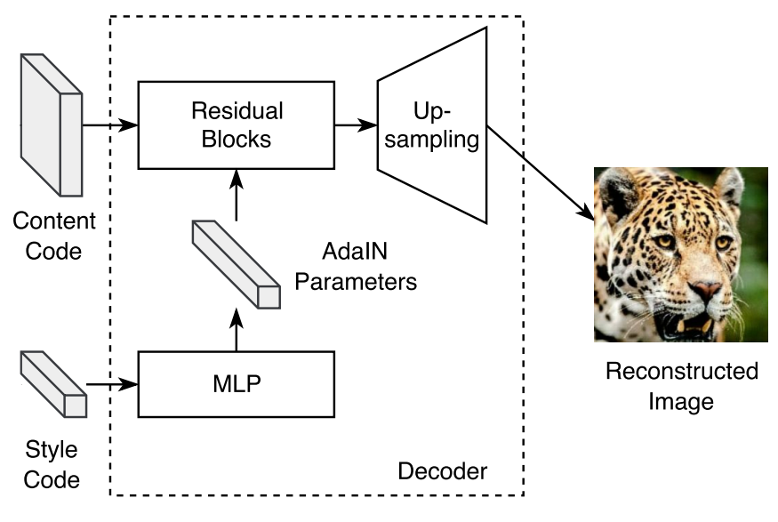
Fig.3에서 표현된 Decoder 부분
Decoder는 Content Encoder, Style Encoder의 결과물인 Content Code와 Style Code를 입력으로 받아 이미지를 생성합니다. Fig.3의 Decoder의 구조에서 Style Code가 MLP를 통과해 AdaIN Parameter를 생성하고 생성된 Parameter가 Residual Blocks에 적용된다 되어 있습니다. Decoder의 핵심인 AdaIN이 뭔데 MLP로 만들고 만들어진 AdaIN Parameter를 Residual Block에 어떻게 적용한다는 건지 그림만으로는 이해하기 어렵습니다. AdaIN에 대해 조금 더 자세하게 알아보겠습니다.
AdaIN (Origin)
\[AdaIN(x, y) = \sigma(y)(\frac{x - \mu(x)}{\sigma(x)}) + \mu(y)\]Style Transfer(1) 글에서 이미지의 style과 content를 분리해 하나의 이미지에 담아내는 것을 이미지 최적화 방법을 통해 구현했었습니다. 하지만 이 방법은 최적화 시간이 오래 걸린다는 단점이 있었는데, AdaIN(Adaptive Instance Normalization)은 이미 학습한 VGG net을 사용한 feature map 입력을 사용해 feature map의 statistic인 평균(mean, $\mu$), 분산(variance, $\sigma$)를 이용해 원하는 style을 feature에 입힐 수 있어 빠르게 Style Transfer가 가능하다는 장점이 있는 방법입니다.
AdaIN을 사용하기 위해서는 우선 Content 이미지와 Style 이미지의 statistic 정보를 가져올 feature map을 추출해야 합니다. 이를 위해 Content 이미지와 Style 이미지를 VGG Encoder(pre-trained VGG)에 입력해 content feature와 style feature를 얻게 되고 이때 content feature가 위 AdaIN 수식의 $x$, style feature가 $y$가 됩니다.
수식에서 $\frac{x - \mu(x)}{\sigma(x)}$는 Standard score Standardization 또는 z-score Standardization이라 불리는 표준화(Standardization) 수식으로 데이터를 정규분포 형태로 바꾸고자 할 때 사용합니다. content feature인 $x$에 대해 z-score를 적용함으로써 $x$에서 style을 제거하고 이후 $\sigma(y)(\frac{x - \mu(x)}{\sigma(x)}) + \mu(y)$로 style feature의 statistics 값을 더해 Style feature인 $y$의 style을 더해줍니다. $\sigma(y)$로 content feature를 scaling하고 $\mu(y)$로 데이터를 shift하는 것으로 style을 표현할 수 있습니다.
Encoder는 pre-trained 모델(VGG-19)이고 AdaIN은 입력받은 feature 간의 statistic를 값을 이용해 feature map $x$를 수정하는 것이 다이기 때문에 learnable parameter가 없다는 것이 특징으로 네트워크에서 학습이 되는 부분은 Decoder만이기 때문에 빠른 학습이 가능합니다.
참고
- Lifeignite / AdaIN을 제대로 이해해보자
AdaIN (MUNIT)
하지만 MUNIT에서는 AdaIN을 조금 다른 방식으로 사용합니다. MLP를 사용해 AdaIN의 parameter를 구하는 방법을 사용하는 것이 차이점입니다. 우선 AdaIN인 AdaptiveInstanceNorm의 코드를 확인해보겠습니다.
class AdaptiveInstanceNorm2d(nn.Module):
    def __init__(self):
        super(AdaptiveInstanceNorm2d, self).__init__()

        self.eps = 1e-5
        self.y_mean = None
        self.y_std = None

    def forward(self, x):
        assert self.y_mean is not None and self.y_std is not None, "Set AdaIN first"

        n, c, h, w = x.size()

        x_mean = x.view(n, c, -1).mean(dim=2).view(n, c, 1, 1).expand(x.size())
        x_var = x.view(n, c, -1).var(dim=2) + self.eps
        x_std = x_var.sqrt().view(n, c, 1, 1).expand(x.size())

        y_mean = self.y_mean.view(n, c, 1, 1).expand(x.size())
        y_std = self.y_std.view(n, c, 1, 1).expand(x.size())

        norm = y_std * ((x - x_mean) / (x_std + self.eps)) + y_mean
        return norm
$x$를 입력으로 받아 $x$의 mean, std를 style feature에 해당하는 $y$로 바꿔주는 norm을 계산해 return합니다. 이때 $y$를 forward에서 입력으로 받아 mean, std를 계산하는 것이 아니라 이미 계산되어 저장된 값을 사용합니다. 이 계산된 값은 어디에서 오나요? 바로 MLP에서 계산되어 옵니다! 기존 AdaIN이 pretrained VGG-19에서 style feature map을 가져와 mean, std를 계산하는 것과는 다르게 MUNIT에서는 Style Encoder로 계산한 Style code를 MLP에 입력으로 넣어 MLP의 결과 값을 style mean, std 값으로 사용합니다. 아직도 왜 MLP를 통해서 계산하는지는 이해하지 못했습니다. 굳이…? 왜….?
AdaIN은 Decoder의 Residual Blocks에 사용되므로 Residual Block 수만큼의 계산된 $y$의 mean, std 값이 필요하겠죠? Decoder 구조는 $\mathsf{R256, R256, R256, R256, u128, u64, c7s1-3}$ 로 총 4개의 Residual block이 사용됩니다. 하나의 Residual Block에는 256개의 channel을 가지고 있고 하나의 Residual Block에 적용되는 AdaIN은 mean, std 2개의 값이 필요하니 Residual Block 당 512개의 값이 필요합니다. Decoder에 사용되는 Residual block은 4개이므로 총 2048개의 값이 MLP를 통해 계산되어야 합니다.
MLP의 입력은 Style Code로 8차원의 벡터 값을 입력으로 받습니다. nn.Linear를 이용해 sample의 size를 필요한 parameter 개수인 2048로 out_feature 수를 맞춰주어 벡터 사이즈를 늘려주었습니다.
class MLP(nn.Module):
    def __init__(self):
        super(MLP, self).__init__()

        self.model = nn.Sequential(
            nn.Linear(8, 256),
            nn.ReLU(),
            nn.Linear(256, 256),
            nn.ReLU(),
            nn.Linear(256, 2048)
        )

    def forward(self, x):
        x = self.model(x)
        return x
MLP를 이용해 계산된 parameter는 decoder를 사용하기 전에 세팅해주어야 합니다. 위의 AdaptiveInstanceNorm2d 코드에서도 forward 함수의 첫 줄은 assert 문으로 만일 parameter(self.y_mean, self.y_std)가 세팅되어 있지 않다면 에러를 출력할 수 있도록 된 것을 보실 수 있습니다. 세팅은 set_adain 함수를 사용합니다. decode 함수에서 mlp에서 계산한 parameter를 받아와 set_adain 함수에 넘깁니다. set_adain 함수에서는 모델의 모든 모듈을 확인하며 AdaptiveInstanceNorm2d 모듈을 발견하면 해당 모듈의 y_mean, y_std에 param을 세팅합니다.
def decode(self, content, style):
    param = self.mlp(style)
    self.set_adain(param)

    return self.decoder(content)


def set_adain(self, param):
    cnt = 0
    for m in self.decoder.modules():
        if m.__class__.__name__ == 'AdaptiveInstanceNorm2d':
            m.y_mean = param[:, cnt*256:(cnt+1)*256]
            m.y_std = param[:, (cnt+1)*256:(cnt+2)*256]
            cnt += 2
class Decoder
Decoder의 구조는 $\mathsf{R256, R256, R256, R256, u128, u64, c7s1-3}$로 Residual, xk 클래스를 사용해 아래와 같이 구현했습니다.
class Decoder(nn.Module):
    def __init__(self):
        super(Decoder, self).__init__()

        self.model = nn.Sequential(
            # Residual
            Residual(256, 256, norm_mode='adain'),
            Residual(256, 256, norm_mode='adain'),
            Residual(256, 256, norm_mode='adain'),
            Residual(256, 256, norm_mode='adain'),

            # Upsampling
            xk('uk', 256, 128),
            xk('uk', 128, 64),

            # c7s1-3
            nn.Conv2d(64, 3, kernel_size=7, stride=1, padding=3, padding_mode='reflect'),
            nn.Tanh()
        )

    def forward(self, x):
        return self.model(x)
Decoder의 Residual은 instance normalization이 아닌 Adaptive Instance Normalization을 사용하므로 norm_mode=’adain’으로 지정해 Residual 객체를 생성했습니다. uk는 up-sampling 과정으로 이미지 크기를 키우고 채널 수를 줄여 최종적으로 이미지를 생성하는 역할을 합니다.
class xk(nn.Module):
    def __init__(self, name, in_feature, out_feature, norm_mode='in'):
        super(xk, self).__init__()

        model = []
        norm = [nn.InstanceNorm2d(out_feature)]
        relu = [nn.ReLU()]

        if name == 'c7s1':
            conv = [nn.Conv2d(in_feature, out_feature, kernel_size=7, stride=1, padding=3, padding_mode='reflect')]

        elif name == 'dk':
            conv = [nn.Conv2d(in_feature, out_feature, kernel_size=4, stride=2, padding=1, padding_mode='reflect')]

        elif name == 'uk':
            conv = []
            conv += [nn.Upsample(scale_factor=2, mode='nearest')]
            conv += [nn.Conv2d(in_feature, out_feature, kernel_size=5, stride=1, padding=2)]

            norm = [LayerNorm(out_feature)]

        model += conv
        model += norm
        model += relu

        self.model = nn.Sequential(*model)

    def forward(self, x):
        return self.model(x)
xk 클래스의 ‘uk’부분에서는 nn.Upsampling과 nn.Conv2d가 번갈아 나오는 것을 볼 수 있습니다. 이는 Checker-board artifact를 감소시키기 위한 방법으로 CycleGAN에서 ConvTranspose2d를 사용해 feature map의 크기를 키우고 channel 수를 줄이는 작업을 했다면 MUNIT에서는 Upsampling과 Conv2d를 사용해 feature map의 크기를 키우고 channel 수를 줄이는 작업을 합니다.
Upsampling을 사용하는 이유는 ConvTranspose2d를 사용했을 때 생기는 artifact를 방지하기 위함입니다. ConvTranspose2d를 사용했을 때 feature map 별 kernel이 overlap 되는 횟수 차이가 발생해 Checkerboard Artifact가 생길 수 있기 때문입니다. Distill의 글에서 Checkerboard Artifact에 대해 더 자세한 설명이 되어 있으니 읽어보시는 것을 추천드립니다.
참고
- Distill / Deconvolution and Checkerboard Artifacts
uk의 normalization은 instance normalization이 아닌 layer normlization을 사용합니다. instance norm은 global feature의 mean, variance를 삭제하기 때문에 style information을 제대로 표현하지 못하므로 LayerNorm을 사용한다는 것을 MUNIT의 issue에서 발견하게 되었습니다. LayerNorm 코드는 공식 코드에서 가져와 사용했습니다.
class LayerNorm(nn.Module):
    def __init__(self, num_features, eps=1e-5, affine=True):
        super(LayerNorm, self).__init__()
        self.num_features = num_features
        self.affine = affine
        self.eps = eps

        if self.affine:
            self.gamma = nn.Parameter(torch.Tensor(num_features).uniform_())
            self.beta = nn.Parameter(torch.zeros(num_features))

    def forward(self, x):
        shape = [-1] + [1] * (x.dim() - 1)

        if x.size(0) == 1:
            # These two lines run much faster in pytorch 0.4 than the two lines listed below.
            mean = x.view(-1).mean().view(*shape)
            std = x.view(-1).std().view(*shape)
        else:
            mean = x.view(x.size(0), -1).mean(1).view(*shape)
            std = x.view(x.size(0), -1).std(1).view(*shape)

        x = (x - mean) / (std + self.eps)

        if self.affine:
            shape = [1, -1] + [1] * (x.dim() - 2)
            x = x * self.gamma.view(*shape) + self.beta.view(*shape)
        return x
Discriminator
Discriminator는 Pix2PixHD의 Multi-scale discriminator를 사용합니다. 고해상도의 이미지를 처리하기 위해 더 깊은 네트워크 또는 더 큰 convolution kernel을 사용하나 두 가지 방법 모두 네트워크 용량을 증가시키고 잠재적으로 overfitting을 유발할 수 있으며 더 큰 메모리 공간을 필요로 한다는 단점을 언급하며 Pix2PixHD에서는 이 문제를 해결하기 위해 multi-scale discriminator를 제안합니다.
Multi scale discriminator는 말그대로 여러 개의 판별 모델을 사용하는 방법입니다. 네트워크 구조(PatchGAN)은 동일하지만 서로 다른 크기의 이미지에서 동작하는 판별 모델을 사용합니다. 원본 이미지 크기에서 동작하는 $D_1$, 원본 이미지의 높이, 너비가 절반이 된 이미지에서 동작하는 $D_2$, 원본 이미지의 높이, 너비가 1/4가 된 이미지에서 동작하는 $D_3$를 사용하며 이때 모든 판별 모델의 구조는 동일합니다.
정말 이미지 크기만 다르게 입력으로 넣게 되면서 $D_1$, $D_2$, $D_3$의 receptive field 크기가 달라지 되는데 가장 큰 receptive field를 가진 $D_1$은 이미지를 전체적으로 보면서 생성 모델이 일관된 이미지를 생성하도록 유도할 수 있으며 가장 작은 $D_3$는 생성 모델이 더 디테일을 생성할 수 있도록 유도할 수 있다고 합니다.
Discriminator의 구조는 CycleGAN - 코드구현의 Discriminator와 광장히 유사합니다. 0.2 slope인 LeakyReLU와 InstanceNorm을 사용하며 convolution의 channel, kernel size, stride, padding 크기 모두 일치합니다. 하지만 모델 마지막의 convolution에 차이가 있습니다.
CycleGAN, Pix2Pix에서는 ConvTranspose2d를 사용해 receptive field 크기를 70x70으로 맞춘 70x70 PatchGAN을 사용했습니다. 하지만 MUNIT에서는 receptive field 크기가 논문에 언급된 것이 없었고 Multi scale discriminator를 사용해 다양한 receptive field를 가진 여러 $D$를 사용하므로 굳이 Convtranspose2d를 사용해 70x70으로 맞출 필요가 사라졌습니다.
따라서 MUNIT에서는 Convtranspose2d를 사용하지 않고 Conv2d로 channel 수를 512에서 1로 만듭니다. Discriminator의 구조를 아래 코드에서 확인하실 수 있습니다.
class Discriminator(nn.Module):
    def __init__(self):
        super(Discriminator, self).__init__()

        self.D1 = self.set_model()
        self.D2 = self.set_model()
        self.D3 = self.set_model()

        self.downsample = nn.AvgPool2d(3, stride=2, padding=1, count_include_pad=False)

    def set_model(self):
        model = nn.Sequential(
            nn.Conv2d(3, 64, kernel_size=4, stride=2, padding=1, padding_mode='reflect'),
            nn.LeakyReLU(0.2),
            nn.Conv2d(64, 128, kernel_size=4, stride=2, padding=1, padding_mode='reflect'),
            nn.InstanceNorm2d(64),
            nn.LeakyReLU(0.2),
            nn.Conv2d(128, 256, kernel_size=4, stride=2, padding=1, padding_mode='reflect'),
            nn.InstanceNorm2d(256),
            nn.LeakyReLU(0.2),
            nn.Conv2d(256, 512, kernel_size=4, stride=2, padding=1, padding_mode='reflect'),
            nn.InstanceNorm2d(512),
            nn.LeakyReLU(0.2),
            nn.Conv2d(512, 1, kernel_size=1)
        )

        return model

    def forward(self, x):
        out_d1 = self.D1(x)
        x = self.downsample(x)
        out_d2 = self.D2(x)
        x = self.downsample(x)
        out_d3 = self.D3(x)

        return [out_d1, out_d2, out_d3]
이미지 크기는 nn.Avgpool2d로 바꿔주며 위 코드의 경우 256 x 256 크기의 이미지가 forward의 x로 들어오면 $D_1$, $D_2$, $D_3$마다 receptive field 크기는 각각 [batch_size, 1, 16, 16], [batch_size, 1, 8, 8], [batch_size, 1, 4, 4]가 됩니다.
class MUNIT
Content Encoder, Style Encoder, Decoder, Discriminator를 편하게 다룰 수 있는 class MUNIT을 구현했습니다.
Adversarial 학습을 하기 때문에 Generator 학습 부분과 Discriminator 학습 부분이 분리 되어 있기에 Generator 학습 시 학습할 parameter 와 Discriminator 학습 시 학습할 parameter를 따로 모아두었습니다. Generator와 관련된 parameter들인 content encoder, style encoder, mlp, decoder의 parameter들을 모아 gen_params으로, discriminator의 parameter를 dis_params으로 선언했습니다.
그 외에도 encode, decode, discriminate 기능을 함수로 만들고 decoder에서 등장했던 set_adain 함수 또한 class MUNIT에 있어 decoder 내부 모듈을 확인 후 AdaIN을 사용하는 모듈에 AdaIN parameter인 y_mean, y_std를 설정할 수 있도록 구현했습니다.
class MUNIT(nn.Module):
    def __init__(self):
        super(MUNIT, self).__init__()

        self.content_encoder = ContentEncoder()
        self.style_encoder = StyleEncoder()
        self.mlp = MLP()
        self.decoder = Decoder()  # Generator
        self.discriminator = Discriminator()

        self.gen_params = list(self.content_encoder.parameters()) + list(self.style_encoder.parameters()) + list(self.mlp.parameters()) + list(self.decoder.parameters())
        self.dis_params = list(self.discriminator.parameters())

    def encode(self, x):
        content = self.content_encoder(x)
        style = self.style_encoder(x)
        return content, style

    def decode(self, content, style):
        param = self.mlp(style)
        self.set_adain(param)

        return self.decoder(content)

    def discriminate(self, x):
        return self.discriminator.forward(x)

    def loss_gan(self, results, target):
        loss = 0

        for result in results:
            loss += torch.mean((result - target) ** 2)

        return loss

    def set_adain(self, param):
        cnt = 0
        for m in self.decoder.modules():
            if m.__class__.__name__ == 'AdaptiveInstanceNorm2d':
                m.y_mean = param[:, cnt*256:(cnt+1)*256]
                m.y_std = param[:, (cnt+1)*256:(cnt+2)*256]
                cnt += 2
3. Loss
Loss는 크게 Adversarial loss, Bidirectional Reconstruction Loss 2가지 종류로 나뉘어집니다. 그리고 Reconstruction Loss는 image reconstruction, style reconstruction, content reconstruction 3가지로 나뉘어집니다.
Reconstruction은 image recon, style recon, content recon으로 나뉘니 각각 loss로 계산될 때 비율을 정해야 하는데 논문에서는 image recon($\lambda_x$) : style recon($\lambda_s$) : content recon($\lambda_c$) = 10 : 1 : 1로 계산합니다.
Adversarial Loss
Adversarial loss로는 CycleGAN 코드 구현글에서도 소개했었던 LSGAN의 목적함수를 사용합니다.
\[\min _D V _{LSGAN}(D) = \frac{1}{2} \mathbb{E} _{x \sim p _{data}(x)}[(D(x) - b) ^2] + \frac{1}{2} \mathbb{E} _{z \sim p _{z}(z)}[(D(G(z)) - a) ^2]\] \[\min _G V _{LSGAN}(G) = \frac{1}{2} \mathbb{E} _{z \sim p _{z}(z)}[(D(G(z)) - c) ^2]\]CycleGAN에서는 nn.MSELoss()를 사용해 구현했었고 이번에는 코드를 짜보았습니다.
def loss_gan(self, results, target):
    loss = 0

    for result in results:
        loss += torch.mean((result - target) ** 2)

    return loss
target 값으로 0 또는 1의 값이 들어오게 되며 results로는 Discriminator의 결과값이 들어오게 됩니다. 두 값의 차이를 제곱한 값을 loss로 사용하는 것은 일치하나 for 문이 추가되어 있는 걸 볼 수 있습니다. Discriminator가 이전의 논문들과는 다르게 Multi-scale로 판별 결과가 3개($D_1$, $D_2$, $D_3$)이기 때문에 for 문을 통해 판별 모델 결과 별 loss를 구하고 더해주었습니다.
Bidirectional Reconstruction Loss
Bidirectional Reconstruction Loss는 Image reconstruction과 Latent reconstruction으로 나뉩니다.
- Image reconstruction : image $\rightarrow$ latent $\rightarrow$ image
- Latent reconstruction : latent $\rightarrow$ image $\rightarrow$ latent
Image reconstruction은 이미지 $x_1$를 encode해 style, content code를 만든 후 두 code를 다시 decode했을 때 결과 이미지 $G_1(E_1(x_1))$와 원본 이미지 $x$ 간의 차이($|G_1(E_1(x_1)) - x_1|_1$)를 계산합니다.
Latent reconstruction은 style reconstruction, content reconstruction이 있으며 latent code($c_1$, $s_2$)를 이용해 decode해 생성한 이미지($G_2(c_1, s_2)$)를 만든 후 해당 이미지를 encode한 결과인 latent code($E_2(G_2(c_1, s_2))$)를 이미지를 만들 때 사용한 latent code와의 차이를 계산합니다. content reconstruction은 $| E ^c _2(G_2(c_1, s_2)) - c_1|_1$, style reconstruction은 $| E ^s _2(G_2(c_1, s_2)) - s_2 |_1$를 계산합니다.
Reconstruction loss는 모두 L1 distance를 계산하기 때문에 pytorch에서 제공하는 nn.L1Loss를 사용해 계산했으며 아래의 코드는 Generator 학습시 사용되는 Reconstruction 계산을 구현한 부분입니다.
loss_l1 = torch.nn.L1Loss()

image_dog = next(iter(dataloader_dog)).cuda()
image_cat = next(iter(dataloader_cat)).cuda()

style_rand_dog = torch.autograd.Variable(torch.randn((1, 8)).cuda())
style_rand_cat = torch.autograd.Variable(torch.randn((1, 8)).cuda())

# encode
content_dog, style_dog = munit_dog.encode(image_dog)
content_cat, style_cat = munit_cat.encode(image_cat)

# decode(differ domain)
recon_dog = munit_dog.decode(content_cat, style_rand_dog)
recon_cat = munit_cat.decode(content_dog, style_rand_cat)

# encode(latent reconstruction)
content_hat_cat, style_hat_rand_dog = munit_dog.encode(recon_dog)
content_hat_dog, style_hat_rand_cat = munit_cat.encode(recon_cat)

recon_latent_c_dog = loss_l1(content_hat_dog, content_dog)
recon_latent_c_cat = loss_l1(content_hat_cat, content_cat)
recon_latent_s_dog = loss_l1(style_hat_rand_dog, style_rand_dog)
recon_latent_s_cat = loss_l1(style_hat_rand_cat, style_rand_cat)
Option
추가로 옵션으로 사용할 수 있는 Loss가 2개 더 있습니다. Domain-inavariant perceptual loss와 Style-augmented cycle consistency loss입니다.
Perceptual loss
perceptual loss는 이전 Munit(1)에서 소개되었었는데, VGG net을 이용해 feature map 간의 거리를 계산한 loss 였습니다. perceptual loss는 고해상도(> 512x512) 이미지 데이터에 효과를 보기 때문에 고해상도 데이터에 적용한다 언급됩니다. 공식 github 코드의 config를 통해 loss의 사용 여부와 loss 간 비율을 알 수 있는데 synthia2cityscape config에서 vgg_w 값이 1로 domain-invariant perceptual loss를 사용하며 이미지 크기가 512x512인 것을 확인할 수 있으며 다른 config에서는 perceptual loss를 사용하지 않음을 확인할 수 있었습니다. 저 또한 이미지 크기가 256x256으로 perceptual loss는 사용하지 않았습니다.
Style cyc loss
Style-augmented cycle consistency loss는 논문에서도 Bidirectional Reconstruction loss와 유사하며 Bidirectional Reconstruction loss에서도 암시되는 내용이라 언급됩니다. 이미 암시되기 때문에 필수로 사용해야 하는 것이 아니고 일부 데이터 셋에서만 명시적으로 사용하는 것이 도움이 될 수 있다고 합니다.
\[\lambda ^{x_1} _{cc} = \mathbb{E} _{x_1 \sim p(x_1), s_2 \sim q(s_2)} [\| G_1(E ^c _2(G_2(E ^c _1(x_1), s_2)), E ^s _1(x_1)) - x_1 \|_1]\]Style-augmented cycle consistency loss는 Latent Reconstruction에서 계산했던 $E ^c _2(G_2(c_1, s_2))$를 사용하기 때문에 코드가 추가되는 부분이 짧습니다. 계산한 $E ^c _2(G_2(c_1, s_2))$와 $s_1$을 decode해 만든 이미지($G_1(E ^c _2(G_2(c_1, s_2)), s_1)$)와 원본 이미지 $x_1$과의 차이를 계산합니다. 추가되는 부분은 아래 코드의 recon_cyc_dog, recon_cyc_cat으로 위 부분의 코드는 latent recon의 코드와 동일합니다.
loss_l1 = torch.nn.L1Loss()

image_dog = next(iter(dataloader_dog)).cuda()
image_cat = next(iter(dataloader_cat)).cuda()

style_rand_dog = torch.autograd.Variable(torch.randn((1, 8)).cuda())
style_rand_cat = torch.autograd.Variable(torch.randn((1, 8)).cuda())

# encode
content_dog, style_dog = munit_dog.encode(image_dog)
content_cat, style_cat = munit_cat.encode(image_cat)

# decode(differ domain)
recon_dog = munit_dog.decode(content_cat, style_rand_dog)
recon_cat = munit_cat.decode(content_dog, style_rand_cat)

# encode(latent reconstruction)
content_hat_cat, style_hat_rand_dog = munit_dog.encode(recon_dog)
content_hat_dog, style_hat_rand_cat = munit_cat.encode(recon_cat)

# decode(cycle consistency)
recon_cyc_dog = munit_dog.decode(content_hat_dog, style_dog)
recon_cyc_cat = munit_cat.decode(content_hat_cat, style_cat)

recon_cyc_dog = loss_l1(recon_cyc_dog, image_dog)
recon_cyc_cat = loss_l1(recon_cyc_cat, image_cat)
모든 데이터셋에 적용한다고 도움이 되는 loss가 아니여서 처음에는 적용하지 않았지만 결과가 좋지 않아 Style_augmented cycle consistency loss를 적용해보았습니다. 저는 적용한 결과가 더 좋다고 느꼈기에 저처럼 MUNIT 논문에서 사용하지 않은 데이터셋을 사용하신다면 적용을 하는 것과 하지 않는 것, 둘 다 테스트 해보시는 것을 추천드립니다.
MUNIT 논문에서 사용한 데이터셋을 사용하신다면 MUNIT 공식 코드의 config를 통해 적용 여부를 확인하실 수 있습니다.
4. 학습
scheduler
논문에서는 100,000 iteration 마다 lr 값이 절반으로 줄어든다 되어 있습니다. AFHQ 데이터셋이 한 epoch 당 약 5,000장 정도이기에 50,000 정도마다 절반씩 줄어드는 것으로 step_size=10, gamma=0.5로 설정한 lr_scheduler.StepLR()을 사용했습니다.
# 결과 부분에서 수정됩니다
scheduler_gen = torch.optim.lr_scheduler.StepLR(optimizer_gen, step_size=10, gamma=0.5)
scheduler_dis = torch.optim.lr_scheduler.StepLR(optimizer_dis, step_size=10, gamma=0.5)
학습
Geneator, Discriminator 학습에 대한 전체 코드입니다.
for epoch in range(n_epoch):
    time_start = datetime.now()
    munit_dog.train()
    munit_cat.train()

    for i in tqdm(range(len(dataloader_dog))):
        image_dog = next(iter(dataloader_dog)).cuda()
        image_cat = next(iter(dataloader_cat)).cuda()

        '''
        Generator
        '''
        optimizer_gen.zero_grad()

        style_rand_dog = torch.autograd.Variable(torch.randn((1, 8)).cuda())
        style_rand_cat = torch.autograd.Variable(torch.randn((1, 8)).cuda())


        # encode
        content_dog, style_dog = munit_dog.encode(image_dog)
        content_cat, style_cat = munit_cat.encode(image_cat)

        # decode(origin domain)
        hat_dog = munit_dog.decode(content_dog, style_dog)
        hat_cat = munit_cat.decode(content_cat, style_cat)

        # decode(differ domain)
        recon_dog = munit_dog.decode(content_cat, style_rand_dog)
        recon_cat = munit_cat.decode(content_dog, style_rand_cat)

        # encode(latent reconstruction)
        content_hat_cat, style_hat_rand_dog = munit_dog.encode(recon_dog)
        content_hat_dog, style_hat_rand_cat = munit_cat.encode(recon_cat)

        # decode(cycle consistency)
        recon_cyc_dog = munit_dog.decode(content_hat_dog, style_dog)
        recon_cyc_cat = munit_cat.decode(content_hat_cat, style_cat)

        # loss_adversarial
        loss_gan = munit_dog.loss_gan(munit_dog.discriminate(recon_dog), 1) + \
                   munit_cat.loss_gan(munit_cat.discriminate(recon_cat), 1)

        # loss_reconstruction
        recon_img_dog = loss_l1(hat_dog, image_dog)
        recon_img_cat = loss_l1(hat_cat, image_cat)
        recon_latent_c_dog = loss_l1(content_hat_dog, content_dog)
        recon_latent_c_cat = loss_l1(content_hat_cat, content_cat)
        recon_latent_s_dog = loss_l1(style_hat_rand_dog, style_rand_dog)
        recon_latent_s_cat = loss_l1(style_hat_rand_cat, style_rand_cat)
        recon_cyc_dog = loss_l1(recon_cyc_dog, image_dog)
        recon_cyc_cat = loss_l1(recon_cyc_cat, image_cat)

        # total loss
        loss_G = loss_gan + lambda_x * (recon_img_dog + recon_img_cat) + \
                 lambda_c * (recon_latent_c_dog + recon_latent_c_cat) + \
                 lambda_s * (recon_latent_s_dog + recon_latent_s_cat) + \
                 lambda_cyc * (recon_cyc_dog + recon_cyc_cat)
        history['G'][epoch] += loss_G.item()

        loss_G.backward()
        optimizer_gen.step()

        '''
        Discriminator
        '''
        optimizer_dis.zero_grad()

        # encode
        content_dog, _ = munit_dog.encode(image_dog)
        content_cat, _ = munit_cat.encode(image_cat)

        # decode(differ domain)
        recon_dog = munit_dog.decode(content_cat, style_rand_dog)
        recon_cat = munit_cat.decode(content_dog, style_rand_cat)

        # loss_adversarial(real image)
        loss_gan_real = munit_dog.loss_gan(munit_dog.discriminate(image_dog), 1) + \
                        munit_cat.loss_gan(munit_cat.discriminate(image_cat), 1)

        # loss_adversarial(fake image)
        loss_gan_fake = munit_dog.loss_gan(munit_dog.discriminate(recon_dog), 0) + \
                        munit_cat.loss_gan(munit_cat.discriminate(recon_cat), 0)

        # total loss
        loss_D = loss_gan_real + loss_gan_fake
        history['D'][epoch] += loss_D.item()

        loss_D.backward()
        optimizer_dis.step()

    '''
    scheduler
    '''
    scheduler_gen.step()
    scheduler_dis.step()

    '''
    history
    '''
    history['lr'].append(optimizer_gen.param_groups[0]['lr'])
    history['G'][epoch] /= len(dataloader_dog)
    history['D'][epoch] /= len(dataloader_dog)

    munit_dog.eval()
    munit_cat.eval()
    with torch.no_grad():
        # encode
        content_dog, style_dog = munit_dog.encode(data_dog)
        content_cat, style_cat = munit_cat.encode(data_cat)

        # decode(differ domain)
        recon_dog = munit_dog.decode(content_cat, style_fix_dog)
        recon_cat = munit_cat.decode(content_dog, style_fix_cat)

        test_dog = get_plt_image(recon_dog[0])
        test_cat = get_plt_image(recon_cat[0])

        test_dog.save('./history/test/dog_' + str(epoch).zfill(3) + '.png')
        test_cat.save('./history/test/cat_' + str(epoch).zfill(3) + '.png')

    '''
    print
    '''
    time_end = datetime.now() - time_start
    print('%2dM %2dS / Epoch %2d' % (*divmod(time_end.seconds, 60), epoch + 1))
    print('loss_G: %.5f, loss_D: %.5f \n' % (history['G'][epoch], history['D'][epoch]))
5. 결과
공식 코드의 config를 확인하면 max_iter: 1,000,000로 제가 사용한 데이터셋으로는 약 200 epoch 정도를 학습해야 합니다. 하지만 사용하는 GPU에서 학습시간이 1 epoch에 1시간 이상으로 학습에 시간이 오래 걸려서 30 epoch만 학습한 결과입니다. 당연히 논문의 결과보다는 좋지 못하지만 30 epoch만으로도 어느 정도 결과 이미지를 확인할 수 있다 정도만으로 봐주시면 좋을 것 같습니다 ![]()
![]()
모든 결과 이미지는 학습에서 사용했던 fixed random vector(style code)를 사용해 변환했습니다.
# 결과 history를 출력하기 위한 fix random style code
style_fix_dog = torch.autograd.Variable(torch.randn((1, 8)).cuda())
style_fix_cat = torch.autograd.Variable(torch.randn((1, 8)).cuda())
시도_1
lambda_x = 10, lambda_s = 1, lambda_c = 1로 설정해 30 epoch을 학습한 결과입니다.
뭔가 열심히 변형하려고 한 흔적은 있지만 이미지의 질감이 blur하게 변하고 눈을 없애버리는 것 말고는 개와 고양이 간의 변환을 느낄 수는 없는 결과가 나왔습니다 ![]()
이미지를 encode한 결과인 style code와 content code로 다시 이미지를 decode한 image reconstruction은 기존 이미지보다 blur하지만 잘 작동됨에 비해 style 변환은 되지 않는다고 느껴 labmda 비율을 조절해 다시 학습을 하는 것으로 결정했습니다.
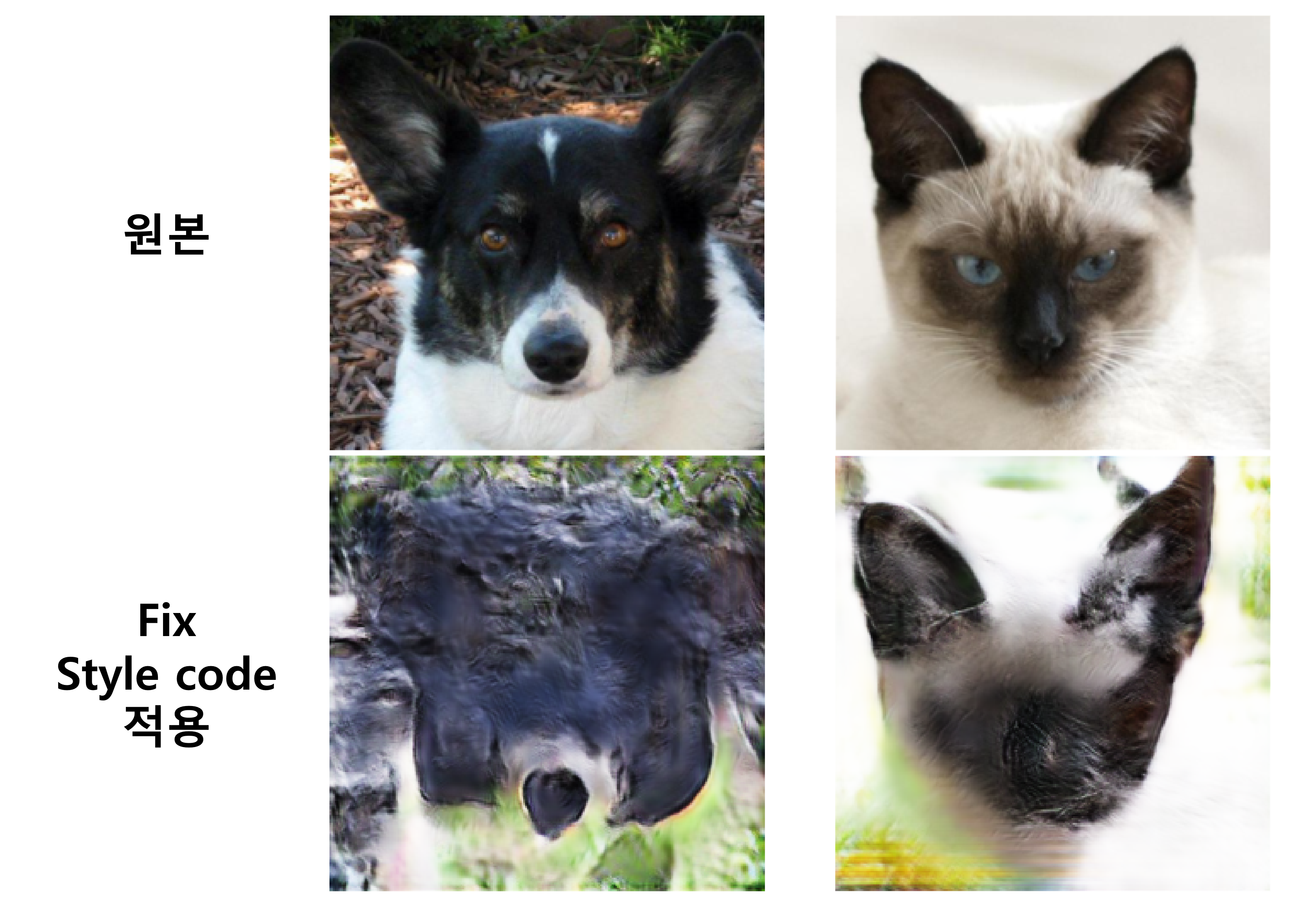
시도_2
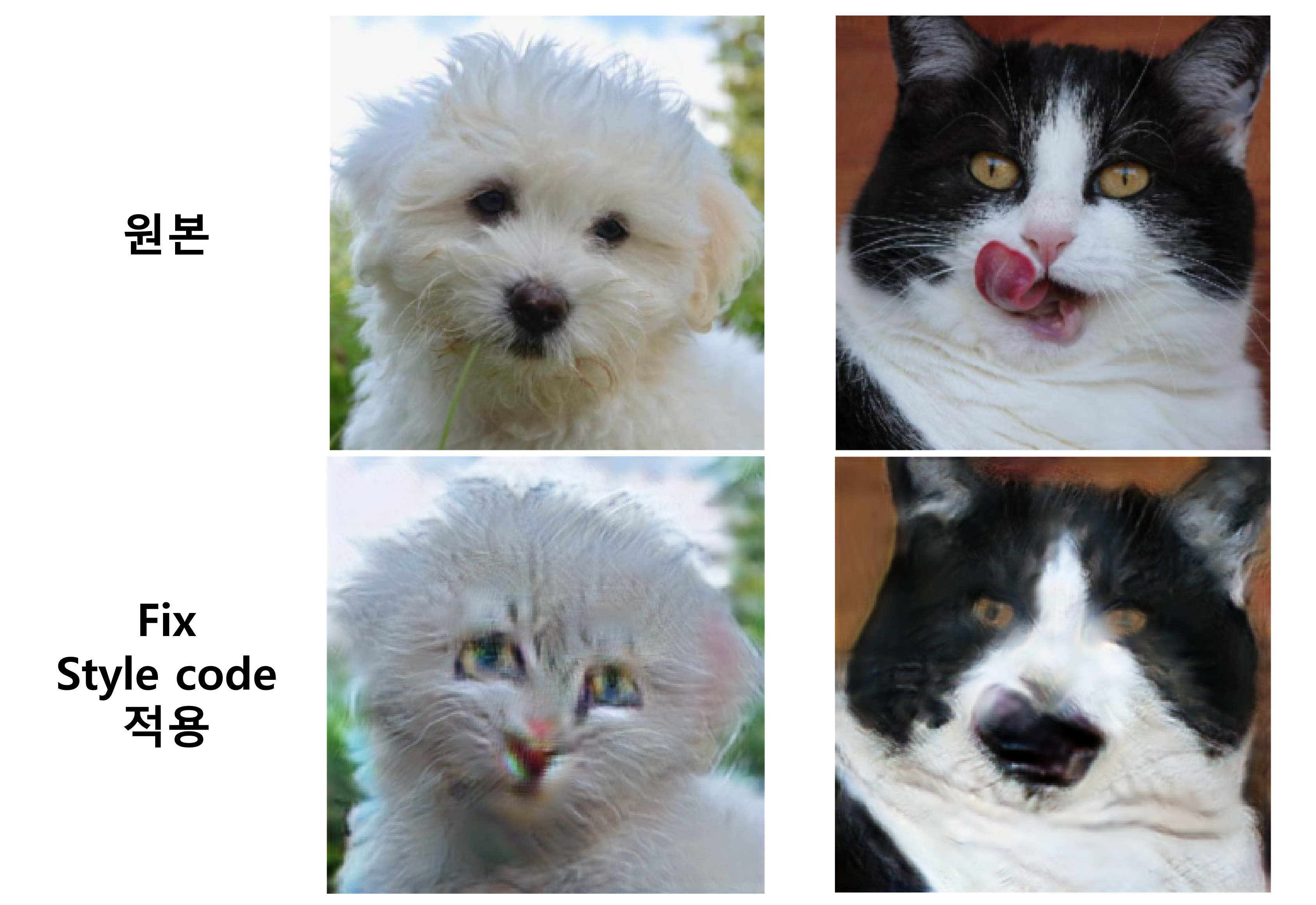
image recon의 비율을 줄이고 style, content recon의 비율을 높여 lambda_x = 7, lambda_s = 3, lambda_c = 3 설정 값을 사용하고 Style-augmented cycle consistency loss를 추가로 사용해 lambda_cyc = 3으로 설정해 30 epoch을 학습한 결과입니다.
오…? 시도_1에 비하면 훨씬 결과가 나아진 것 같습니다. 일단 눈이 확인 가능하네요 ![]()
개 $\rightarrow$ 고양이의 결과 이미지는 꽤 그럴싸하다고 생각했습니다. 코와 입의 모양이 고양이처럼 변했으며 모양이 뚜렷하지는 않지만 눈 또한 고양이 눈으로 변한 것, 그리고 고양이 특유의 긴 흰 수염이 생성됨을 볼 수 있습니다.
하지만 고양이 $\rightarrow$ 개의 결과 이미지는 굳이 따지자면 고양이라 보여집니다. 고양이의 귀가 흐릿해져있으며 눈은 이도저도 아닌 모습이 보여집니다. 하지만 고양이의 흰 수염은 사라지고 코의 모양이 개처럼 변한 것을 볼 수 있었습니다. 개와 고양이를 코와, 턱, 입과 같은 하관으로 구별하나? 라는 생각이 든 결과였습니다. 고양이 $\rightarrow$ 개의 결과를 개선하고자 한번 더 시도를 해보았습니다.
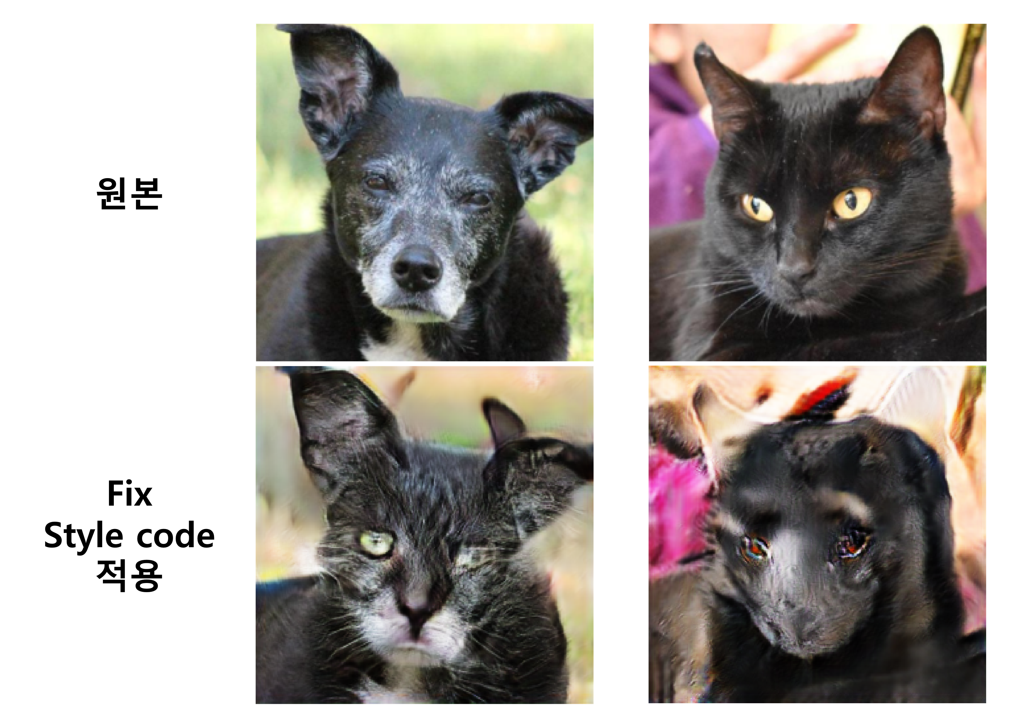
시도_3
lambda_cyc를 추가해 효과를 보았으니 이번에는 lambda_cyc 값을 키워 lambda_cyc = 10으로 설정했습니다. lambda_x, lambda_s, lambda_c의 값은 시도_2와 마찬가지로 각각 7, 3, 3입니다. 또한 scheduler의 step_size를 변경했습니다.
논문은 100,000의 step_size를 가지니 저의 데이터셋의 epoch으로는 약 20 epoch이였고 그 절반 값인 10 epoch을 step_size로 설정해놓았었습니다. 학습 epoch 수가 30 epoch으로 작다보니 step_size도 작아져야겠다 판단해 step_size = 3으로 변경해 다시 시도해보았습니다.
오묘…하지만 시도_2보다 고양이 $\rightarrow$ 개 의 결과가 자연스러워졌습니다!
개 $\rightarrow$ 고양이는 시도_2와 큰 차이를 느끼지는 못했습니다. 눈이 고양이 눈으로, 코와 입이 고양이 코와 입으로 그리고 고양이 특유의 흰 수염이 생김을 볼 수 있습니다. 왠지 비웃는 표정인 것 같은 건 기분 탓이겠죠…?
고양이 $\rightarrow$ 개의 결과는 시도_2보다 더 좋은 결과를 보여주고 있다 생각했습니다. 시도_2는 귀 부분이 흐릿하게 변하며 윤곽이 변했지만 시도_3은 윤곽이 변하지 않았고 눈, 코, 입 부분을 집중적으로 바꾸려 시도한다 느껴졌습니다. 눈의 동공 부분이 조금 더 크고 또렸해졌으며 코와 입 부분이 고양이의 핑크색이 아닌 개의 검은색으로 변한 것을 볼 수 있습니다. 고양이의 혀가 나와있는 이미지라 그런가 혀까지 개의 코로 변환하는 것을 시도했지만 실패한 것 같습니다…![]()
결과의 결과
결과들이 사실 논문에 비하면 나오지 않았지만 포스팅용 이미지를 PPT로 제작하던 중 신기한 걸 발견했습니다. 시도_2, 시도_3의 결과를 PowerPoint는 제가 의도한 대로 Dog $\rightarrow$ Cat을 시도한 이미지는 고양이로, Cat $\rightarrow$ Dog를 시도한 이미지는 개로 인식합니다!
PowerPoint가 인정한 개와 고양이 입니다 ![]()
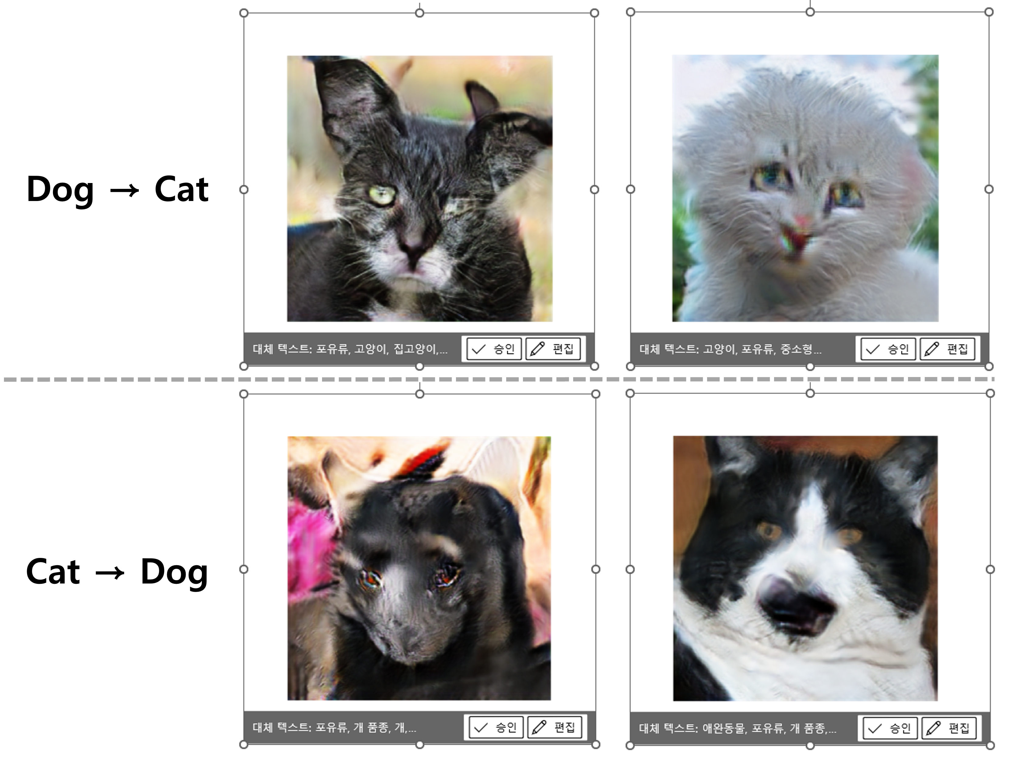
개에서 고양이로 변환한 결과는 고양이로, 고양이에서 개로 변환한 결과는 개로 인식함을 대체 텍스트를 통해 확인할 수 있었습니다.
위 이미지는 PPT에 이미지를 삽입할 때 PPT는 이미지에 대해 자동으로 대체 텍스트 생성하는데, 그 대체 텍스트를 캡쳐한 것입니다. 대체 텍스트가 인식하는 결과를 보니
사실 시도_2의 Cat $\rightarrow$ Dog 결과는 사람이 본다면 고양이로 인식할 거 같은데 개로 인식하는 것이 신기하네요. 정말 하관 부분을 중요포인트로 여기는 게 아닐까 다시 한번 생각했습니다.
얼레벌레 MUNIT 구현 글이 끝났습니다!
지금까지 코드 구현은 그리 무겁지 않아 가능한 한 논문의 조건을 따라 갔었는데 MUNIT 부터는 데탑 성능의 한계가 느껴집니다 ![]()
제가 사용한 데이터셋을 기준으로 논문이 200 epoch 즈음인데 저는 30 epoch 만을 학습했으니 학습의 반의 반도 못 한게 되어버렸네요…. 이것도 하루 넘게 학습을 돌린 건데 조금 슬퍼집니다 어헝헝. 논문 구현에 대한 고민을 조금 더 해봐야 될 것 같습니다 ![]()
이번 글도 끝까지 봐주셔서 감사합니다! 구현에 사용한 코드는 github에서 확인하실 수 있습니다 :)